View the code used in this post on Github
View my overview of Generative Adversarial Networks on YouTube
1. Introduction:
Generative Adversarial Network (GAN) is a machine learning framework that learns from training data and generates new data with the same properties as the training data [1]. For example, a GAN can be trained on images of human faces and generate new images that look like a human face. Look at the following website to see examples of a GAN generated person: https://thispersondoesnotexist.com

Progress of GAN results between 2014-2017. Source: Malicious Use of Artificial Intelligence paper, 2018.
GANs can be applied to generate many types of data including generative art, imagery, modelling scientific problems, early diagnosis, designing new medicines, calculating risk and much more.
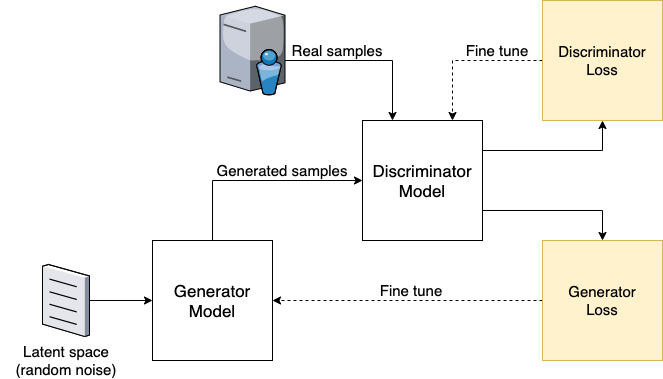
The way that a GAN achieves the result of generating new data is by using two neural network models:
The first is the generator network which generates new samples
The second is the discriminator network which is a binary classifier that classifies whether a sample is real or fake after being given a combination of real training samples and fake generated samples.
The power of GANs lies in the adversarial relationship between generator and discriminator networks.
The generator is always trying to succeed at tricking the discriminator into believing its fake sample are real.
If the discriminator correctly recognises that the fake sample is fake then the generator can take that feedback through its loss function, update the weights of the generator model using backpropagation and try again with a new and better sample.
The discriminator network is also improving at working out which sample is fake using its own loss function.
This relationship leads to a positive feedback loop where the fake samples become more realistic over many iterations and the discriminator becomes harder to trick with fake samples.
Below is a visualisation of how this network architecture looks:
2. Architecture of GAN discriminator and generator models
Now we have a basic understanding of how these models fit together we should turn to a deeper analysis of each of the models that we want to create.
It is important to know there is no one way of building generator and discriminator models, because there are many types of models that suit these roles and a big part of the current state of machine learning is the rapid evolution of models over time that dramatically shift the GAN results. For this module we will focus on the high level architecture that underpins GAN and provide further reading below.
Discriminator model:
The goal of this model is to estimate the probability of given sample x being real and fake, for example, the discriminator might output [0.79, 0.21] meaning there is a 79% chance sample x is real and 21% chance it is fake.
The process for running this model is as follows:
- Input a combination of real and fake samples into the model.
- The discriminator classifies the samples as real or fake with a binary probability distribution of each sample being real or fake.
- The loss is calculated using the discriminator’s loss function.
- Update the discriminator’s weights through backpropagation using gradient descent that we have discussed already in this unit.
- Repeat the process again with new samples.
Generator model:
The goal of this model is to generate fake data. We can think of these as synthetic data points. The overall goal of the generator model is to learn the distribution and boundaries between classes and become better at generating fake samples.
The process for running this model is as follows:
- Select a random seed for the model which is essentially a noise factor, this random seeds helps avoid overfitting and allows some randomness in the final result.
- Generate a random sample and output this into the discriminator network which classifies the sample as real or fake.
- The loss is calculated using the generator’s loss function and is a measure of how successful it was at tricking the discriminator.
- Update the weights of the generator through backpropagation using gradient descent discussed earlier.
- Repeat the process again with new samples.
Latent space: these are the random vector of values / noise that we take as input into the generator model [2]. The important thing about this latent space is that after the generator model has been trained these random values take on meaning as a compressed representation of the output assigned by the model, which means that selecting a specific random value from the latent space will lead to a specific output based on the weights of the generator model.
Loss function of the GANs:
The loss function is what defines the feedback loop of the GANs adversarial networks [3]. We need the discriminator to maximise the loss while the generator will try to minimise the loss.
In the original paper that defined GANs in 2014 the loss function was defined as L = Ex[log(D(x))] + Ez[log(1 – D(G(z)))] where:
D(x) is the discriminator’s probability estimate that real data sample x is real
Ex is the expected value over all real data instances
G(z) is the generator’s output given some noise factor z
D(G(z)) is the discriminator’s probability estimate that fake data sample G(z) is real
Ez is the expected value over all fake data instances
This loss function represents the cross-entropy between real and fake samples, which is a qualification of the difference between both probability distributions.
Note: that the generator cannot directly affect the log(D(x)) term and can only really minimise the log(1 – D(G(z))) which is important to understand that is really what is being minimised by the generator.
Training process:
We should not update the weights of both networks in each epoch otherwise it would be too hard to understand what is happening in the network. Therefore, we should keep the weights of the discriminator static while the generator’s weights are updating and vice versa as follows:
Train the discriminator for a specific number of epochs and freeze / not update the generator’s weights.
Then switch to freezing the discriminator’s weights while we train the generator for a specific number of epochs.
Convergence:
One major issue with GANs is that the discriminator will have diminishing returns as the generator creates more realistic samples [4]. In general a discriminator should converge on loss of 0.5 which is a 50% chance of determining if a sample is real of fake. This 0.5 loss means that the sample is so good it is indistinguishable from something real. The major issue is that if we keep training the discriminator or do not architect or networks properly the GAN results can become worse or unstable as the adversarial networks try to achieve higher success rates. Specific issues we need to look out for include:
Mode collapse: this is where the generator model fails to generalise or learns only a subset of the classes. The reasons for this can be varied such as the architecture of the model, choice of loss function and more.
Failure to converge: this is when there is no balance between generator and discriminator models. This can happen if the generator is outputting too many unrealistic samples when the discriminator’s level of confidence is high leading it to reject the samples of the generator and then causing a vanishing gradient (error is increasing exponentially causing results that are not improving).
3. Understanding GANs through a real-world example
To understand the concepts of GANs more deeply we can look at a basic example of using a GAN to generate handwritten digits. The dataset used is the MNIST dataset of 60,000 handwritten digits [5]. After loading the dataset we can see the digits look like this:
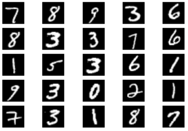
The goal of our GAN is to produce fake samples of digits to trick the discriminator into thinking these digits are real. Below is an explanation of how the program works.
Section 1: we load the dataset and do some exploratory analysis of the data to understand our dataset contains 60,000 images of size 28 x 28 pixels.
import numpy as np
import matplotlib.pyplot as plt
import random

# Import the handwritten digits dataset
from keras.datasets.mnist import load_data

# Import the Keras functionality we need
from tensorflow.keras.optimizers import Adam
from keras.layers import Input, Dense, Reshape, Flatten, Dropout
from keras.layers import BatchNormalization, Activation, ZeroPadding2D
from keras.layers.advanced_activations import LeakyReLU
from keras.layers.convolutional import UpSampling2D, Conv2D
from keras.models import Sequential, Model

# Get the real training data
(X_train, _), (_, _) = load_data()

# Visualise the size/shape of the dataset
print(f"Data shape {X_train.shape}")

# Plot a random sample of 25 numbers to visualise the data
for i in range(25):
    plt.subplot(5, 5, i + 1)
    plt.axis(False)
    plt.imshow(X_train[random.randint(0,99)], cmap='gray')

plt.show()
Section 2: we define the discriminator model, which is the binary classification model we use for deciding if a given sample is real or fake.
This model is a neural network consisting of 3 dense layers, the idea behind the network is to reduce the network input (an image) down to the final probability output.
We use LeakyReLU activation function between layers. ReLU is a linear activation function defined as y = max(0, x), that will output the input if positive or 0 if negative. LeakyReLU improved on ReLU by outputting a small slope instead of 0 if the value is negative e.g. 0.01 instead of 0.
Sigmoid activation is used on the final dense layer as it works well with probability distributions as an output because sigmoid exists between 0 to 1.
We use the binary version of the cross-entropy loss function (discussed earlier) because we are determining between real and fake samples and our model uses this binary loss to fine tune the network.
# Binary classifier used to decide if a given input is real or fake
def discriminator_model(image_shape):
    # This model is a simple 3 dense layer neural network
    model = Sequential()

    model.add(Flatten(input_shape=image_shape))
    model.add(Dense(512, activation=LeakyReLU(alpha=0.2)))
    model.add(Dense(256, activation=LeakyReLU(alpha=0.2)))
    # sigmoid provides output 0 - 1 which is ideal for binary classification
    model.add(Dense(1, activation='sigmoid'))

    model.summary()

    model.compile(loss='binary_crossentropy',
        optimizer=Adam(0.0002, 0.5), metrics=['accuracy'])

    return model
Section 3: we define the generator model which is the model used to generate fake samples of data.
This model takes a random set of values from the latent space (random noise) and outputs the image of size image_shape (width, height and greyscale).
We use batch normalisation before the final dense layer to standardise the activation from the previous layer and stabilise the output of the network [6].
- At a high-level batch normalisation works by normalising the output from the activation of the previous layer as follows: x = (x – μ) / σ where μ is the mean of the output values and σ is the standard deviation of the output values. The normalisation process then multiplies and add the output to two trainable arbitrary parameters which has the effect of reducing the effect of large outlier weights which makes training faster and more stable [7].
Lastly, this model uses the Tanh activation function which is similar to Sigmoid however it outputs values between -1 to 1 which accounts for the range of normalised greyscale values of the image.
# Takes in noise from the latent space and generates fake samples of data
def generator_model(latent_space, image_shape):
    model = Sequential()

    model.add(Dense(256, input_dim=latent_space, activation=LeakyReLU(alpha=0.2)))
    model.add(Dense(512, activation=LeakyReLU(alpha=0.2)))
    model.add(Dense(1024, activation=LeakyReLU(alpha=0.2)))
    model.add(BatchNormalization(momentum=0.8))
    # tanh provides output -1 - 1 which is ideal for our image
    model.add(Dense(np.prod(image_shape), activation='tanh'))
    model.add(Reshape(image_shape))

    model.summary()

    return model
Section 4: we combine our models into a single GAN
We set the discriminator to be non-trainable (we can unlock this later when we want to train the discriminator).
We then initialise all 3 models: discriminator, generator and GAN combined models with a latent space of size 128 (which could be any size really).
def GAN_models(latent_space):
    image_size = 28 # 28 x 28 final image
    num_channels = 1 # network expects a 3D image (28, 28, 1)
    image_shape = (image_size, image_size, num_channels)

    # Initialise generator model
    generator = generator_model(latent_space, image_shape)

    # Initialise discriminator model
    discriminator = discriminator_model(image_shape)

    # Freeze the weights of discriminator and unlock when we need to train
    discriminator.trainable = False

    # The generator's input is noise from the latent space
    inputs = Input(shape=(latent_space,))
    image = generator(inputs)

    # The discriminator's input is image data from the generator
    output = discriminator(image)

    # Combine generator and descriminator models to make the full GAN
    gan = Model(inputs, output)
    gan.compile(loss='binary_crossentropy', optimizer=Adam(0.0002, 0.5))

    return generator, discriminator, gan

latent_space = 128 # Random values / noise vector size

# Initialise our models
generator, discriminator, gan = GAN_models(latent_space)
Section 5: lastly, we train the GAN and plot the results, using the following process:
We scale the training data to have 3 axis (width, height and greyscale)
Then for each epoch we do the following tasks:
Get a random set of real training images of a given batch size (we train in batches).
Get a random set of noise from the latent space of given batch size
Use this noise to create a random set of fake images from the generator model
Combine the real and fake data into a training dataset
Train the discriminator model on this dataset and get the loss value from the loss function.
Train the generator by running the full GAN with discriminator set as non-trainable, this will have the effect of training the generator only.
Periodically save the results from the generator and loss results so we can view and understand the results from the GAN.
def train_model(generator, discriminator, gan, X_train, latent_space, epochs):

    batch_size = 128 # Train in batches of 128
    sample_interval = 100
    print_interval = 25
    discriminator_loss = []
    generator_loss = []

    # Scale training data for (width, height, greyscale) on each image
    X_train = X_train / 127.5 - 1.
    X_train = np.expand_dims(X_train, axis=3)

    for epoch in range(epochs):

        # Step 1: training the discriminator model

        # Get a random set of real images
        image_batch = X_train[np.random.randint(0, X_train.shape[0], batch_size)]

        # Generate a set of noise from the latent space
        noise = np.random.normal(0, 1, (batch_size, latent_space))

        # Generate new set of fake digits
        generated_images = generator.predict(noise)

        # Combine our real and fake data into a training dataset
        X = np.concatenate((image_batch, generated_images))
        y = np.zeros(batch_size * 2) # labels
        y[:batch_size] = 1

        # Unfreeze weights and train the discriminator on combined dataset
        discriminator.trainable = True
        d_loss = discriminator.train_on_batch(X, y)

        # Freeze the weights of the discriminator again so we can train the generator
        discriminator.trainable = False

        # Step 2: training the generator model

        # Generate noise from the latent space
        noise = np.random.normal(0, 1, (batch_size, latent_space))

        # Run GAN with discriminator set as not-trainable to train only the generator
        y2 = np.ones(batch_size) # labels
        g_loss = gan.train_on_batch(noise, y2)

        # Periodically plot the training progress
        if epoch % print_interval == 0:
            print(f"{epoch} => d loss: {d_loss[0]}, g loss: {g_loss}")
            discriminator_loss.append(d_loss[0])
            generator_loss.append(g_loss)

        # Periodically plot the generated images
        if epoch % sample_interval == 0:
            plot_generated(generated_images, epoch)

    # Plot the loss of the discriminator and generator at the end
    plot_loss(discriminator_loss, generator_loss)


def plot_generated(generated_images, epoch):
    # 5 x 5 grid
    rows, columns = 5, 5
    # Scale the generated images
    generated_images = 0.5 * generated_images + 0.5

    # Plot the images onto a 5 x 5 grid
    fig, axs = plt.subplots(rows, columns)
    count = 0
    for i in range(rows):
        for j in range(columns):
            axs[i,j].imshow(generated_images[count, :,:,0], cmap='gray')
            axs[i,j].axis('off')
            count += 1
    # Save the images into a /results/ folder
    fig.savefig("results/%d.png" % epoch)
    plt.close()

# Plot the discriminator and generator loss
def plot_loss(discriminator_loss, generator_loss):
    plt.figure()

    plt.plot(discriminator_loss, label="Discriminator loss")
    plt.plot(generator_loss, label="Generator loss")

    plt.ylabel('Loss Values')
    plt.xlabel('Epochs')

    plt.legend()
    plt.show()

# Train the model and view the results
epochs = 20000
train_model(generator, discriminator, gan, X_train, latent_space, epochs)
The results from our example GAN:
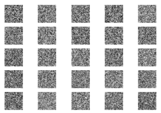
- Before training (epoch 1, starting off with random noise):
- After 30,000 epochs of training:
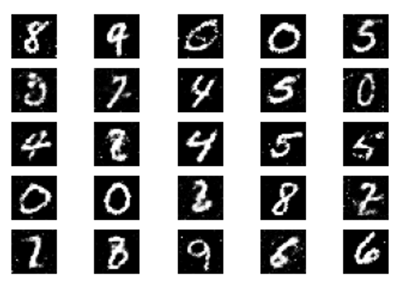
The loss results are close to what we want with the discriminator loss: 0.598241, which is to say that the model is performing well with the loss of the discriminator being close to 50%.
We can also plot the loss of the discriminator and generator to see how the model improves over time:
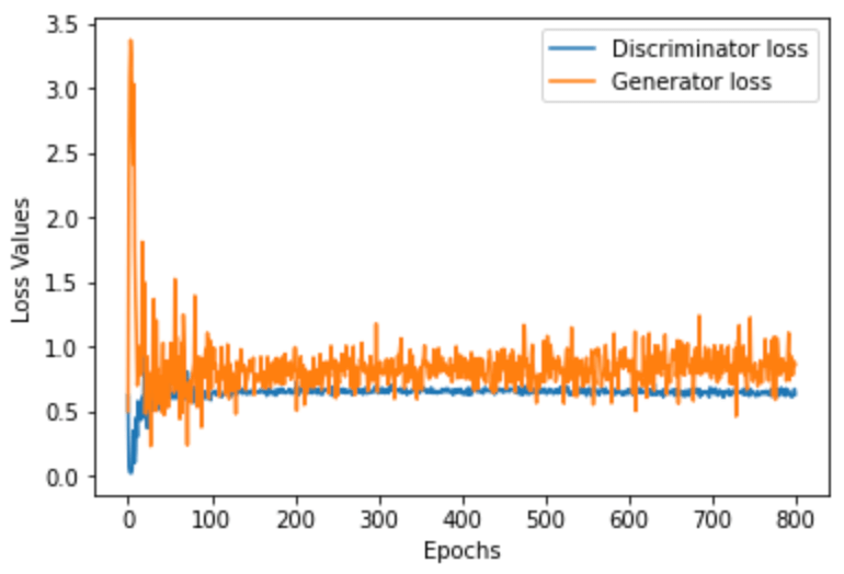
As you can see here, the discriminator settles on a loss of around 0.6 which is roughly consistent with what we wanted to see (having an approximately 50/50 chance of correctly identifying a given data sample) and the generator settles on a loss of around 0.8 – 0.9 which is showing that the generator is quite successful at tricking the discriminator within the margin of 0.2 – 0.1.
View the following video to get a deeper understanding of how the example code works: view video
Additional reading:
[0] Get the code used in this post: https://github.com/joshanthony/generative-adversarial-networks
[1] Generative Adversarial Nets: https://arxiv.org/pdf/1406.2661.pdf
[2] Interpreting the Latent Space of Generative Adversarial Networks using Supervised Learning: https://arxiv.org/pdf/2102.12139.pdf
[3] Generative Adversarial Networks: https://developers.google.com/machine-learning/gan
[4] On convergence and stability of GANs: https://arxiv.org/pdf/1705.07215.pdf
[5] MNIST dataset: http://yann.lecun.com/exdb/mnist
[6] On the Effects of Batch and Weight Normalization in Generative Adversarial Networks: https://arxiv.org/abs/1704.03971
[7] Batch Normalisation Explained: https://www.youtube.com/watch?v=dXB-KQYkzNU

