

Linear regression helps us predict the output of continuous data. For example, it helps us predict the cost of a house or the impact of different types of exercise on a person’s weight.
Today we will be looking at how to perform linear regression to predict a person’s weight based on the type and quantity of exercise they do. We will do this by using the Linnerud dataset which is build into the scikit-learn Python library and available to use as a test dataset.
This is a great way to learn linear regression using one of the most popular machine learning libraries. After reading this article you should be able to apply these same concepts to more complicated datasets.
1. Starting out
To get started all you need is Python, a text editor (or notebook) and a few Python libraries.
import numpy as np
from sklearn import datasets
from sklearn import linear_model
import matplotlib.pyplot as plt

%matplotlib inline
You can find most of these packages through a quick Google Search or below:
From here you load the dataset and set up a few variables to load our dataset and get out X and Y data:
linnerud = datasets.load_linnerud()
chins = linnerud['data'][:,0].reshape(-1,1)
weight = linnerud['target'][:,0].reshape(-1,1)
We have selected the “chins” column of data and we want to see if we can predict a person’s weight based on how many chin-ups they can do.
You can also print out the data to get an idea of what we are actually looking at:
print(linnerud['feature_names'])
print(linnerud['target_names'])
You should see something like:
{% raw %}['Chins', 'Situps', 'Jumps']
['Weight', 'Waist', 'Pulse']{% endraw %}
This is a small dataset and we are only going to work with 2 of these 6 columns of data, how small is our data? Well we can check like so:
print(len(chins))This should print out “20” samples (I told you it was small!)
In practice you would be working with thousands or even millions of rows of data but for our purposes we are learning scikit so this size dataset is fine for us.
Now that we have inspected the size and shape of our data we should plot our data to see if we can see a rough correlation between “chins” and “weight”.
fig, ax = plt.subplots()
plt.figure(figsize=(10,10))
ax.scatter(chins, weight, c='b')
ax.set_title('Chin-ups and weight dependency preview')
ax.set_xlabel('Chin-ups')
ax.set_ylabel('Weight')
plt.show()
The output should look something like this:
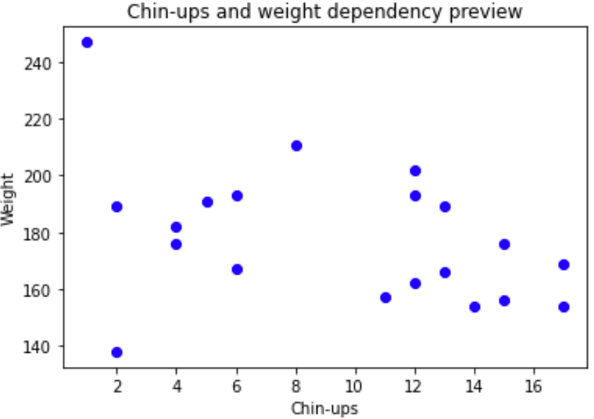
The data looks good! We can see there is an approximate negative correlation between “chins” and “weight” meaning if a person can do more chin-ups, their weight is likely to be smaller.
2. Set up the training and testing data
Next we need to split the data into a training and test dataset so that our model can train on some data and make a prediction and then we can visualise as a test to see how accurate that data is. In this case we choose 70% set aside for training and 30% for testing, this is a pretty standard split between training and testing.
# Calculate the number of samples needed:
n_train = int(len(weight) * 0.7)

# Select the first 70% of data for training
x_train = chins[: n_train]
y_train = weight[: n_train]

# Select the remaining data for testing
x_test = chins[n_train :]
y_test = weight[n_train :]
Now the data is set up and ready to create a linear regression model!
3. Creating our linear regression model
Creating the model is relatively straightforward if you use scikit, you can do it like this:
# Create the model
lr = linear_model.LinearRegression()

# Fit our model to the training data:
lr.fit(x_train, y_train)

# Then predict the Y axis value for our X axis test data:
y_pred = lr.predict(x_test)
4. Visualising the model
Lastly we would like to visualise our data to see if our model is close to our test data:
fig, ax = plt.subplots(figsize=(5, 5), dpi=100)
ax.scatter(x_train, y_train, c='b')
ax.scatter(x_test, y_test, c='g')
ax.plot(x_test, y_pred)

for i in range(len(x_test)):
    plt.plot([x_test[i], x_test[i]], [y_test[i], y_pred[i]], color='g', linewidth=0.5)

ax.set_title('Simulated data and estimated line for Chins vs Weight')
ax.set_xlabel('Chins')
ax.set_ylabel('Weight')
plt.show()
This gives us our training data in blue, our test data is green and our linear regression model in a blue line.
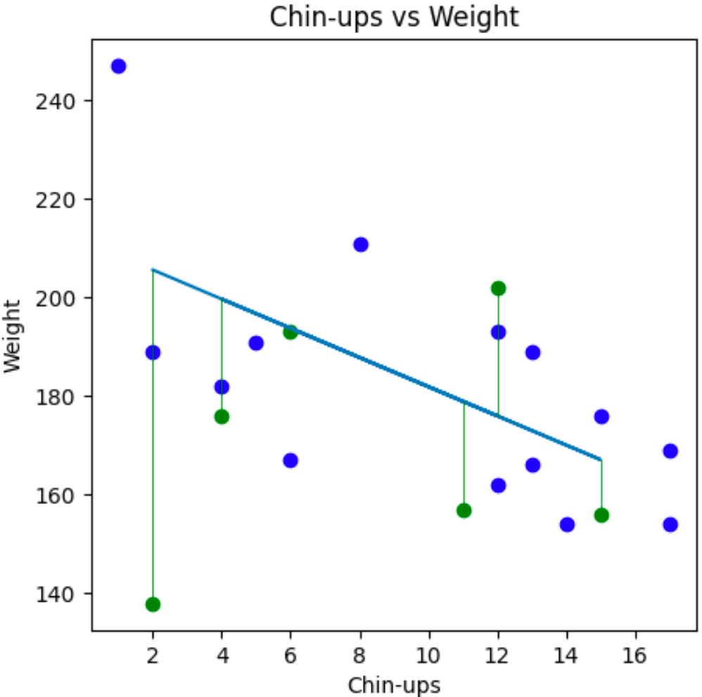
We can see that our linear regression model line more of less fits the same slope as the training and testing data so we can say, yes our model appears to be accurate for the data we have.
5. Checking the accuracy of our model
One way to test the accuracy of our data is to check the Pearson correlation coefficient like this:
pearson_coeff = np.corrcoef(chins, weight)
print(pearson_coeff)
This will give us a score between -1 and 1 where 1 is a strong positive correlation, -1 is a strong negative correlation and 0 is no correlation. There is a bunch of mathematics that relates to this which is very interesting and should be discussed another time.
Here we can see that we have a -0.389 Pearson correlation coefficient score which means there is a small negative correlation (as chins go up, weight goes down). The conclusion we can make here is that the data doesn’t fit that well but it is giving us something that roughly looks like dependency, which is good enough for our learning purposes.
Strong dependency can be hard to find depending on the data you work with you might not find any dependency.
Wait, but what happens if my line does not fit the training and test data?
There are many reasons for this. Sometimes data has no correlation and therefore we cannot easily fit a linear regression model. That is perfectly fine! It is reasonable to sometimes conclude that something does not relate to another thing.
Lack of correlation can also be valuable, for example if a company thinks some new type of safety gear will have a positive impact on safety and your model proves that it does not affect safety then that means you have done a great thing with your model by reducing the waste of time and resources.
That’s it! We have now created our first linear regression model and visualised it. I hope this helps!